Approximate Bayesian Inference¶

Below is a quick example of how to use approxposterior to estimate an accurate approximation to the posterior distribution of the Rosenbrock Function example from Wang & Li (2018) using the BAPE algorithm. In many Bayesian inference applications, sampling methods used to derive posterior distributions, such as Markov Chain Monte Carlo (MCMC) methods, can require >1,000,000 functions evaluations. In cases where the forward model is computationally expensive, such methods quickly become infeasible. The active learning approach employed by approxposterior, however, requires orders of magnitude fewer simulations to train approxposterior’s GP, yielding accurate approximate Bayesian posterior distributions.

Note that setting verbose = True also outputs additional diagnostic information, such as when the MCMC finishes, what the estimated burn-in is, and other quantities that are useful for tracking the progress of your code. In this example, we set verbose = False for simplicity.

First, the user must set model parameters.

from approxposterior import approx, gpUtils, likelihood as lh, utility as ut
import numpy as np

# Define algorithm parameters
m0 = 50                           # Initial size of training set
m = 20                            # Number of new points to find each iteration
nmax = 2                          # Maximum number of iterations
bounds = [(-5,5), (-5,5)]         # Prior bounds
algorithm = "bape"                # Use the Kandasamy et al. (2017) formalism
seed = 57                         # RNG seed
np.random.seed(seed)

# emcee MCMC parameters
samplerKwargs = {"nwalkers" : 20}        # emcee.EnsembleSampler parameters
mcmcKwargs = {"iterations" : int(2.0e4)} # emcee.EnsembleSampler.run_mcmc parameters

Create an initial training set and gaussian process

# Sample design points from prior
theta = lh.rosenbrockSample(m0)

# Evaluate forward model log likelihood + lnprior for each theta
y = np.zeros(len(theta))
for ii in range(len(theta)):
    y[ii] = lh.rosenbrockLnlike(theta[ii]) + lh.rosenbrockLnprior(theta[ii])

# Default GP with an ExpSquaredKernel
gp = gpUtils.defaultGP(theta, y, white_noise=-12)

Initialize the approxposterior object.

# Initialize object using the Wang & Li (2018) Rosenbrock function example
ap = approx.ApproxPosterior(theta=theta,                     # Initial model parameters for inputs
                            y=y,                             # Logprobability of each input
                            gp=gp,                           # Initialize Gaussian Process
                            lnprior=lh.rosenbrockLnprior,    # logprior function
                            lnlike=lh.rosenbrockLnlike,      # loglikelihood function
                            priorSample=lh.rosenbrockSample, # Prior sample function
                            algorithm=algorithm,             # bape, agp, jones, or alternate
                            bounds=bounds)                   # Parameter bounds

Run!

# Run!
ap.run(m=m, nmax=nmax, estBurnin=True, nGPRestarts=3, mcmcKwargs=mcmcKwargs,
       cache=False, samplerKwargs=samplerKwargs, verbose=True, thinChains=False,
       onlyLastMCMC=True)

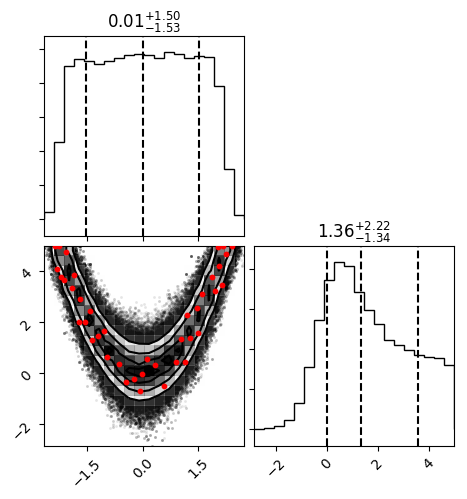
Examine the final posterior distributions

# Check out the final posterior distribution!
import corner

# Load in chain from last iteration
samples = ap.sampler.get_chain(discard=ap.iburns[-1], flat=True, thin=ap.ithins[-1])

# Corner plot!
fig = corner.corner(samples, quantiles=[0.16, 0.5, 0.84], show_titles=True,
                    scale_hist=True, plot_contours=True)

fig.savefig("finalPosterior.png", bbox_inches="tight")

The final posterior distribution will look something like the following:

Check the notebook below to see MCMC sampling with using the Rosenbrock function and emcee.

Jupyter Notebook Examples:

Rosenbrock Function Example