Fitting a Line

---

In this notebook, we reproduce the classic “Fitting a Model to Data” example from emcee, https://emcee.readthedocs.io/en/latest/tutorials/line/, fitting a line with uncertainties, using both emcee and approxposterior. This notebook demonstrates how approxposterior can be used to perform accurate Bayesian inference of model parameters given data with uncertainties.

import numpy as np
import matplotlib.pyplot as plt
import emcee
from scipy.optimize import minimize
import corner
import george

from approxposterior import approx, gpUtils as gpu

Data

---

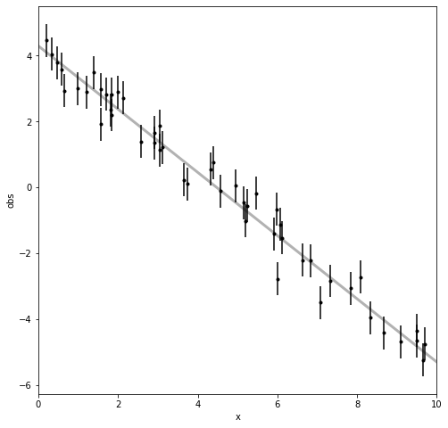
First, we generate data according to \(y_i = m * x_i + b + \epsilon_i\) where \(\epsilon_i\) are indepedent, Gaussian errors, for each measurement \(i\). Then we’ll plot the data to see what it looks like, with the grey line being the true, underlying model.

# Set seed for reproducibility.
seed = 42
np.random.seed(seed)

# Choose the "true" parameters.
mTrue = -0.9594
bTrue = 4.294

# Generate some synthetic data from the model.
N = 50
x = np.sort(10*np.random.rand(N))
obserr = 0.5 # Amplitude of noise term
obs = mTrue * x + bTrue # True model
obs += obserr * np.random.randn(N) # Add some random noise

# Now plot it to see what the data looks like
fig, ax = plt.subplots(figsize=(8,8))

ax.errorbar(x, obs, yerr=obserr, fmt=".k", capsize=0)
x0 = np.linspace(0, 10, 500)
ax.plot(x0, mTrue*x0+bTrue, "k", alpha=0.3, lw=3)
ax.set_xlim(0, 10)
ax.set_xlabel("x")
ax.set_ylabel("obs");

Inference

---

Now we want to infer posterior probability distributions for our linear model’s parameters, \(\theta\), i.e slope and intercept, given the data and uncertainties, D, via Bayes’ Theorem: \(p(\theta | D) \propto l(D | \theta)p(\theta)\) where \(l(D|\theta)\) is the likelihood of the data for a given set of model parameters, and \(p(\theta)\) is our assume prior probability of a given \(\theta\). We sample the posterior distribution using the emcee MCMC code. See the emcee example (https://emcee.readthedocs.io/en/latest/tutorials/line/) for more details of this procedure.

# Define the loglikelihood function
def logLikelihood(theta, x, obs, obserr):

    # Model parameters
    theta = np.array(theta)
    m, b = theta

    # Model predictions given parameters
    model = m * x + b

    # Likelihood of data given model parameters
    return -0.5*np.sum((obs-model)**2/obserr**2)

# Define the logprior function
def logPrior(theta):

    # Model parameters
    theta = np.array(theta)
    m, b = theta

    # Probability of model parameters: flat prior
    if -5.0 < m < 0.5 and 0.0 < b < 10.0:
        return 0.0
    return -np.inf

# Define logprobability function: l(D|theta) * p(theta)
# Note: use this for emcee, not approxposterior!
def logProbability(theta, x, obs, obserr):

    lp = logPrior(theta)
    if not np.isfinite(lp):
        return -np.inf
    return lp + logLikelihood(theta, x, obs, obserr)

Now that we’ve set up the required functions, we initialize our MCMC sampler in emcee, pick an initial state for the walkers, and run the MCMC!

# Randomly initialize walkers
p0 = np.random.randn(32, 2)
nwalkers, ndim = p0.shape

# Set up MCMC sample object - give it the logprobability function
sampler = emcee.EnsembleSampler(nwalkers, ndim, logProbability, args=(x, obs, obserr))

# Run the MCMC for 5000 iteratios
sampler.run_mcmc(p0, 5000);

/opt/anaconda3/lib/python3.7/site-packages/emcee/moves/red_blue.py:99: RuntimeWarning: invalid value encountered in double_scalars
  lnpdiff = f + nlp - state.log_prob[j]

The MCMC is complete, so let’s examine the joint and marginal posterior probability distributions it derived for the model parameters.

fig = corner.corner(sampler.flatchain,
                    quantiles=[0.16, 0.5, 0.84],
                    truths=[mTrue, bTrue],
                    labels=["m", "b"], range=([-1.1,-0.8],[3.7, 4.8]),
                    plot_contours=True, show_titles=True);

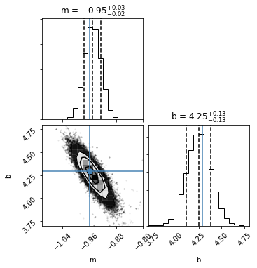
Looks good!

Inference with ``approxposterior``

---

Now let’s see if we can derive similar constraints using approxposterior.

First, approxposterior requires a function that samples model parameters from the prior distributions.

def sampleFunction(n):
    """
    docs

    Parameters
    ----------
    n : int
        Number of samples

    Returns
    -------
    sample : floats
        n x 3 array of floats samples from the prior
    """

    # Sample model parameters given prior distributions
    m = np.random.uniform(low=-5, high=0.5, size=(n))
    b = np.random.uniform(low=0, high=10, size=(n))

    return np.array([m,b]).T
# end function

Define the approxposterior parameters.

# Define algorithm parameters
m0 = 20                           # Initial size of training set
m = 10                            # Number of new points to find each iteration
nmax = 5                          # Maximum number of iterations
bounds = [(-5,0.5),(0.0,10.0)]    # Prior bounds
algorithm = "bape"                # Use the Kandasamy et al. (2017) formalism

# emcee MCMC parameters: Use the same MCMC parameters as the emcee-only analysis
samplerKwargs = {"nwalkers" : 32}  # emcee.EnsembleSampler parameters
mcmcKwargs = {"iterations" : 5000} # emcee.EnsembleSampler.run_mcmc parameters

# Data and uncertainties that we use to condition our model
args = (x, obs, obserr)

Here we create the initial training set by running the true forward model \(m_0\) times. approxposterior learns on this training set and, each iteration, runs the forward model \(m\) additional times in regions of parameter space that will most improve its owns predictive performance, iteratively improving the posterior distribution estimate.

# Create a training set to condition the GP

# Randomly sample initial conditions from the prior
theta = np.array(sampleFunction(m0))

# Evaluate forward model to compute log likelihood + lnprior for each theta
y = list()
for ii in range(len(theta)):
    y.append(logLikelihood(theta[ii], *args) + logPrior(theta[ii]))
y = np.array(y)

# We'll create the initial GP using approxposterior's built-in default
# initialization.  This default typically works well in many applications.
gp = gpu.defaultGP(theta, y)

Now initialize the ApproxPosterior object and we’re ready to go!

ap = approx.ApproxPosterior(theta=theta,                   # Initial model parameters for inputs
                            y=y,                           # Logprobability of each input
                            gp=gp,                         # Initialize Gaussian Process
                            lnprior=logPrior,              # logprior function
                            lnlike=logLikelihood,          # loglikelihood function
                            priorSample=sampleFunction,    # Prior sample function
                            algorithm=algorithm,           # bape, agp, or alternate
                            bounds=bounds)                 # Parameter bounds

Run approxposterior! Note that we set cache to False so approxposterior only saves the most recent sampler and MCMC chain instead of saving each full MCMC chain to a local HD5f file (see emcee v3 documentation for more details on how emcee caches data).

# Run!
ap.run(m=m, nmax=nmax,estBurnin=True, mcmcKwargs=mcmcKwargs, cache=False,
       samplerKwargs=samplerKwargs, verbose=False, args=args, onlyLastMCMC=True,
       seed=seed)

As before, let’s plot the joint and marginal posterior probability distributions to see how approxposterior did. In addition, as red points, we’ll plot where approxposterior decided to evaluate the forward model to improve its own performance. As you’ll see below, approxposterior preferentially runs the forward model in regions of high posterior probability density - it doesn’t waste time on low likelihood regions of parameter space!

samples = ap.sampler.get_chain(discard=ap.iburns[-1], flat=True, thin=ap.ithins[-1])

fig = corner.corner(samples, quantiles=[0.16, 0.5, 0.84], truths=[mTrue, bTrue],
                    labels=["m", "b"], show_titles=True, scale_hist=True,
                    plot_contours=True, range=([-1.1,-0.8],[3.7, 4.8]));

# Plot where forward model was evaluated
fig.axes[2].scatter(ap.theta[:,0], ap.theta[:,1], s=8, color="red", zorder=20);

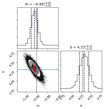
The predictions are close to the true MCMC!