MAP Estimation
approxposterior can be used to find an accurate approximation of the
maximum (or minimum) of a function by estimating the maximum a
posteriori (MAP) solution for the objective function. To find the MAP, we directly
maximize the GP surrogate model’s posterior function, that is, the approximation
to the objective function learned by the GP after conditioning on observations. By design,
approxposterior trains its Gaussian process (GP) on a small number of
objective function evaluations. This method is therefore particularly useful
when the objective function is computationally-expensive to evaluate.
Below is a quick example of how to use approxposterior to estimate the
MAP solution of a simple 2D Gaussian.
In this case, we are using the -loglikelihood function of a 2D Gaussian with a mean
vector of 0 and the identity matrix as the covariance matrix. The MAP solution
we find using approxposterior is therefore the minimum. We hope to
recover the global minimum of 0 at (0,0), but only using 10 randomly sampled
points to make our training set for the GP.
First, the user must set model parameters.
from approxposterior import approx, gpUtils, likelihood as lh, utility as ut
import numpy as np

# Define algorithm parameters
m0 = 10                           # Size of training set
bounds = ((-5,5), (-5,5))         # Prior bounds
algorithm = "bape"                # Use the Kandasamy et al. (2017) formalism
seed = 57                         # RNG seed
np.random.seed(seed)
Create an initial training set and Gaussian process
# Sample design points from prior
theta = lh.sphereSample(m0)

# Evaluate forward model log likelihood + lnprior for each point
y = np.zeros(len(theta))
for ii in range(len(theta)):
    y[ii] = lh.sphereLnlike(theta[ii]) + lh.sphereLnprior(theta[ii])

# Initialize default gp with an ExpSquaredKernel
gp = gpUtils.defaultGP(theta, y, white_noise=-12, fitAmp=True)
Initialize the
approxposteriorobject and optimize GP hyperparameters
# Initialize approxposterior object
ap = approx.ApproxPosterior(theta=theta,
                            y=y,
                            gp=gp,
                            lnprior=lh.sphereLnprior,
                            lnlike=lh.sphereLnlike,
                            priorSample=lh.sphereSample,
                            bounds=bounds,
                            algorithm=algorithm)

# Optimize the GP hyperparameters
ap.optGP(seed=seed, method="powell", nGPRestarts=1)
Find MAP solution
# Find MAP solution and function value at MAP
MAP, val = ap.findMAP(nRestarts=5)
Compare
approxposteriorMAP solution to truth: 0 at (0,0)
# Plot MAP solution on top of grid of objective function evaluations
import matplotlib.pyplot as plt

fig, ax = plt.subplots(figsize=(7,6))

# Generate grid of function values the old fashioned way because this function
# is not vectorized...
arr = np.linspace(-2, 2, 100)
sphere = np.zeros((100,100))
for ii in range(100):
    for jj in range(100):
        sphere[ii,jj] = lh.sphereLnlike([arr[ii], arr[jj]])

# Plot objective function (rescale because it varies by several orders of magnitude)
ax.imshow(np.log(-sphere).T, origin="lower", aspect="auto", interpolation="nearest",
          extent=[-2, 2, -2, 2], zorder=0, cmap="viridis_r")

# Plot truth
ax.axhline(0, lw=2, ls=":", color="white", zorder=1)
ax.axvline(0, lw=2, ls=":", color="white", zorder=1)

# Plot MAP solution
ax.scatter(MAP[0], MAP[1], color="red", s=50, zorder=2)

# Format figure
ax.set_xlabel("x0", fontsize=15)
ax.set_ylabel("x1", fontsize=15)
title = "MAP estimate, value: (%0.3lf, %0.3lf), %e\n" % (MAP[0], MAP[1], val)
title += "Global minimum coords, value: (%0.1lf, %0.1lf), %d\n" % (0.0, 0.0, 0)
ax.set_title(title, fontsize=12)

# Save figure
fig.savefig("map.png", bbox_inches="tight")
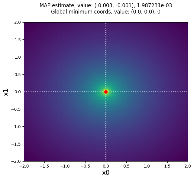
approxposterior MAP solution: (-0.003 -0.001), 0.00198723 (red point),
compared to the truth (0,0), 0 (white dashed lines).
Our answer is pretty close to the truth, and better yet, approxposterior
only required 10 randomly-distributed objective function evaluations to train
its GP used to estimate the MAP solution. For computationally-expensive
forward models, this method can be used for efficient (approximate) Bayesian
optimization of functions. Better yet, MAP estimation can be ran after intelligently
expanding the GP’s training set with the run or bayesOpt methods, or after calling
findNewPoint! See the detailed API for how to use those functions.