True Rosenbrock Posterior Calculation Using Emcee

---

David P. Fleming, 2019

This notebook demonstrates how to use the Metropolis-Hastings MCMC algorithm to derive the posterior distribution for the Rosenbrock function example presented in Wang & Li (2017) using emcee.

See https://emcee.readthedocs.io/en/stable/ for more information on emcee.

%matplotlib inline

from approxposterior import likelihood as lh
from approxposterior import mcmcUtils

import numpy as np
import emcee
import corner
import matplotlib as mpl
import matplotlib.pyplot as plt
mpl.rcParams.update({'font.size': 18})

np.random.seed(42)

Set up MCMC initial conditions

---

ndim = 2          # Number of dimensions
nsteps = 20000    # Number of MCMC iterations

nwalk = 20 * ndim # Use 20 walkers per dimension

# Initial guess for walkers (random over prior)
p0 = [lh.rosenbrockSample(1) for j in range(nwalk)]

Initialize MCMC Ensemble Sampler object

---

Note that here, we use the lh.rosenbrock_lnprob function that computes the log-likelihood plus the log-prior for the Rosenbrock function model as described in Wang & Li (2017). The functions used to compute this example is provided in approxposterior. See example.py in approxposterior’s examples directory for to see how approxposterior’s BAPE algorithm approximates the Rosenbrock function posterior derived in this notebook.

sampler = emcee.EnsembleSampler(nwalk, ndim, lh.rosenbrockLnprob)

Run the MCMC!

---

After the MCMC run finishes, we estimate the burn in following the example in the emcee documentation.

sampler.run_mcmc(p0, nsteps)
print("emcee finished!")

emcee finished!

# Compute acceptance fraction for each walker
print("Number of iterations: %d" % sampler.iteration)

# Is the length of the chain at least 50 tau?
print("Likely converged if iterations > 50 * (integrated autocorrelation time, tau).")
print("Number of iterations / tau:", sampler.iteration / sampler.get_autocorr_time(tol=0))

Number of iterations: 20000
Likely converged if iterations > 50 * (integrated autocorrelation time, tau).
Number of iterations / tau: [152.45258457 288.91391155]

iburn = int(2.0*np.max(sampler.get_autocorr_time(tol=0)))
print(iburn)

262

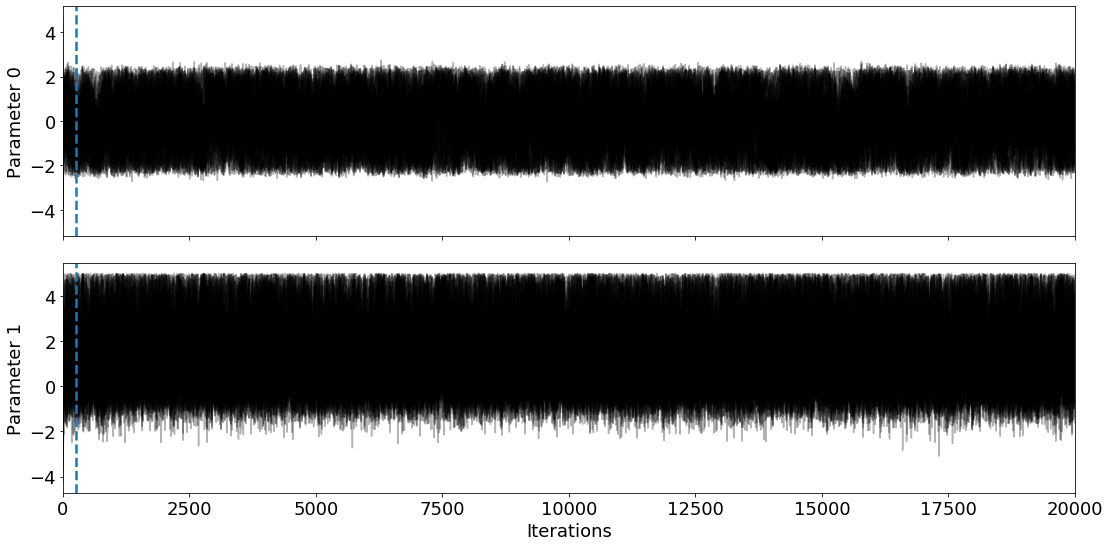
Let’s visually inspect the chains to see if they’re converged.

---

The blue dashed line corresponds to our burn in estimate.

fig, ax = plt.subplots(nrows=2, sharex=True, figsize=(16,8))

# Plot allllll the walkers and chains
ax[0].plot(sampler.chain[:,:,0].T, '-', color='k', alpha=0.3);
ax[1].plot(sampler.chain[:,:,1].T, '-', color='k', alpha=0.3);

# Plot where the burn in is
ax[0].axvline(iburn, ls="--", color="C0", lw=2.5)
ax[1].axvline(iburn, ls="--", color="C0", lw=2.5)

# Formatting
ax[0].set_xlim(0,nsteps)
ax[1].set_xlim(0,nsteps)
ax[0].set_ylabel("Parameter 0")
ax[1].set_ylabel("Parameter 1")
ax[1].set_xlabel("Iterations")

fig.tight_layout()

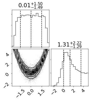
Looks good! Let’s plot the joint and marginal posterior distributions.

---

fig = corner.corner(sampler.get_chain(discard=iburn, flat=True, thin=int(iburn/4.0)),
                    quantiles=[0.16, 0.5, 0.84],
                    plot_contours=True, show_titles=True);

fig.savefig("true_post.pdf", bbox_inches="tight")

Neat. Now let’s save the sampler object and burn in time into a numpy archive so we can compare our approximate distributions with the truth derived here to see how accurate approxposterior (in another notebook…)!

np.savez("trueRosenbrock.npz",
         flatchain=sampler.flatchain,
         iburn=iburn)