Bayesian Optimization

approxposterior can be used to find an accurate approximation to the maximum (or minimum) of an expensive objective function using Bayesian optimization. As is common in modern Bayesian optimization applications, approxposterior trains a Gaussian process (GP) surrogate model for the objective function on a small number of function evaluations. approxposterior then maximizes a utility function, here Jones et al. (1998)’s “Expected Utility”, to identify where to next observe the objective function. In this case, the Expected Utility function attempts to strike a balance between “exploration” and “exploitation”, as it seeks to find where observing the objective function will improve the current estimate of the maximum, or at least improve the surrogate model’s estimate of the objective function.

This method is particularly useful when the objective function in question is computationally-expensive to evaluate, so one wishes to minimizes the number of evaluations. For some great reviews on the theory of Bayesian Optimization and its implementation, check out: this great blog post by Martin Krasser and this excellent review paper by Brochu et al. (2010).

Below is an example of how to use approxposterior to estimate the maximum of a 1D function with Bayesian Optimization and maximum a posteriori (MAP) estimation using the function learned by GP surrogate model. For the MAP estimation, approxposterior directly maximizes the GP surrogate model’s posterior function, that is, the approximation to the objective function learned by the GP after conditioning on observations.

Note that in general, approxposterior wants to maximize functions since it is designed for approximate probabilistic inference (e.g., we are interested in maximum likelihood solutions), so keep this in mind when coding up your own objective functions. If you’re instead interested in minimizing some function, throw a - sign in front of your function. Finally, note that in approxposterior, we defined objective functions as the sum of a loglikelihood function and a logprior function. Typically, the loglikelihood function is simply the objective function. The logprior function can encode any prior information the user has about the objective, but here we use it to enforce a simple uniform prior with hard bounds over the domain [-1,2].

For this example, we wish to find the maximum of the following objective function:

# Plot objective function
fig, ax = plt.subplots(figsize=(6,5))

x = np.linspace(-1, 2, 100)
ax.plot(x, lh.testBOFn(x), lw=2.5, color="k")

# Format
ax.set_xlim(-1.1, 2.1)
ax.set_xlabel(r"$\theta$")
ax.set_ylabel(r"f($\theta$)")

# Hide top, right axes
ax.spines["right"].set_visible(False)
ax.spines["top"].set_visible(False)
ax.yaxis.set_ticks_position("left")
ax.xaxis.set_ticks_position("bottom")

fig.savefig("objFn.png", bbox_inches="tight", dpi=200)

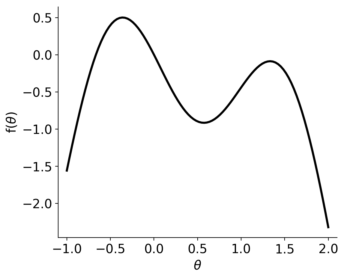
This objective function has a clear global maximum, but also a local maximum, so it should be a reasonable test. Now to the optimization.

1. First, the user must set model parameters.

# Define algorithm parameters
m0 = 3                           # Size of initial training set
bounds = [[-1, 2]]               # Prior bounds
algorithm = "jones"              # Expected Utility from Jones et al. (1998)
numNewPoints = 10                # Maximum number of new design points to find
seed = 91                        # RNG seed
np.random.seed(seed)

2. Create an initial training set and Gaussian process

# Sample design points from prior to create initial training set
theta = lh.testBOFnSample(m0)

# Evaluate forward model + lnprior for each point
y = np.zeros(len(theta))
for ii in range(len(theta)):
    y[ii] = lh.testBOFn(theta[ii]) + lh.testBOFnLnPrior(theta[ii])

# Initialize default gp with an ExpSquaredKernel
gp = gpUtils.defaultGP(theta, y, white_noise=-12, fitAmp=True)

3. Initialize the approxposterior object, optimize GP hyperparameters

# Initialize object using a simple 1D test function
ap = approx.ApproxPosterior(theta=theta,
                            y=y,
                            gp=gp,
                            lnprior=lh.testBOFnLnPrior,
                            lnlike=lh.testBOFn,
                            priorSample=lh.testBOFnSample,
                            bounds=bounds,
                            algorithm=algorithm)

# Optimize the GP hyperparameters
ap.optGP(seed=seed, method="powell", nGPRestarts=1)

4. Perform Bayesian Optimization

# Run the Bayesian optimization!
soln = ap.bayesOpt(nmax=numNewPoints, tol=1.0e-3, kmax=3, seed=seed, verbose=False,
                   cache=False, gpMethod="powell", optGPEveryN=1, nGPRestarts=2,
                   nMinObjRestarts=5, initGPOpt=True, minObjMethod="nelder-mead",
                   gpHyperPrior=gpUtils.defaultHyperPrior, findMAP=True)

The soln dictionary returned by ap.bayesOpt contains several parameters, including the solution path, soln["thetas"], and the value of the function at each theta, soln["vals"], along the solution path. soln["thetaBest"] and soln["valBest"] give the coordinates and function value as the inferred maximum, respectively.

This Bayesian optimization routine will run for up to nmax iterations, or until the best solution changed by <= tol for kmax consecutive iterations. In this case, only 9 iterations were ran, so the solution converged at the specified tolerance. Additionally, by setting optGPEveryN = 1, we re-optimized the GP hyperparameters each time approxposterior added a new point to its training set by maximizing the Expected Utility function. Keeping optGPEveryN to low values will tend to produce more accurate solutions as, especially for early iterations, the GP’s posterior function can change quickly as it gains more information as the training set expands.

In addition to finding the Bayesian optimization solution, we set findMAP=True to have approxposterior also find the maximum a posteriori (MAP) solution. That is, the approxposterior identified the maximum of the posterior function learned by the GP. This optimization is rather cheap since it does not require evaluating the forward model. Since approxposterior’s goal is to have its GP actively learn an approximation to the objective function, its maximum should be approximately equal to the true maximum. soln contains the MAP solution path, soln["thetasMAP"], the value of the GP posterior function at each theta along the MAP solution path, soln["valsMAP"], the MAP solution, soln["thetaMAPBest"], and the GP posterior function value at the MAP, soln["valMAPBest"].

Below, we’ll compare the Bayesian optimization and MAP solution paths contained in soln.

5. Compare approxposterior BayesOpt, MAP solution to truth:

import matplotlib
import matplotlib.pyplot as plt
matplotlib.rcParams.update({"font.size": 15})

# Plot the solution path and function value convergence
fig, axes = plt.subplots(ncols=2, figsize=(12,6))

# Extract number of iterations ran by bayesopt routine
iters = [ii for ii in range(soln["nev"])]

# Left: solution
axes[0].axhline(trueSoln["x"], ls="--", color="k", lw=2)
axes[0].plot(iters, soln["thetas"], "o-", color="C0", lw=2.5, label="GP BayesOpt")
axes[0].plot(iters, soln["thetasMAP"], "o-", color="C1", lw=2.5, label="GP approximate MAP")

# Format
axes[0].set_ylabel(r"$\theta$")
axes[0].legend(loc="best", framealpha=0, fontsize=14)

# Right: solution value (- true soln since we minimized -fn)
axes[1].axhline(-trueSoln["fun"], ls="--", color="k", lw=2)
axes[1].plot(iters, soln["vals"], "o-", color="C0", lw=2.5)
axes[1].plot(iters, soln["valsMAP"], "o-", color="C1", lw=2.5)

# Format
axes[1].set_ylabel(r"$f(\theta)$")

# Format both axes
for ax in axes:
    ax.set_xlabel("Iteration")
    ax.set_xlim(-0.2, soln["nev"]-0.8)

    # Hide top, right axes
    ax.spines["right"].set_visible(False)
    ax.spines["top"].set_visible(False)
    ax.yaxis.set_ticks_position("left")
    ax.xaxis.set_ticks_position("bottom")

fig.savefig("bo.png", dpi=200, bbox_inches="tight")

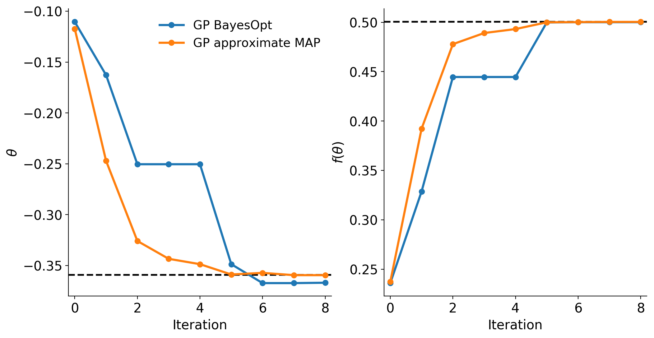
Using Bayesian optimization, approxposterior estimated the maximum of the objective function to be (-0.367, 0.500), compared to the truth, (-0.359, 0.500), represented by the black dashed lines in both panels. Looks pretty good! approxposterior found an MAP solution of (-0.360, 0.500), slighty better than the Bayesian optimization solution. As seen in the figure above, both the Bayesian optimization and GP MAP solutions quickly converge to the correct answer. Since approxposterior continues to re-train and improve the GP’s posterior predictive ability as the training set expands, its MAP solution actually converges to the correct answer more quickly than Bayesian optimization. Note that this is not expected in general, but can be used to efficiently estimate extrema.