Hierarchical Bayesian analysis of the 2019-2020 NHL season (until it got suspended)
I miss hockey, so I decided to build a simple hierarchical Bayesian model to simulate the remainder of the 2019-2020 NHL season. Since this model is data-driven and fully probabilistic, I will be able to quantify the offensive and defensive ability of teams given the games they have already played this season. NHL coaches could then use these insights to help inform gameplans for a given opponent. Furthermore, I can draw samples from the posterior distribution to simulate entire seasons to see which teams likely make the playoffs.
This work is based in large part on Baio and Blangiardo, Daniel Weitzenfeld’s great write-up, and a nice application of this type of modeling to Rugby from the PyMC3 docs.
Summary of the main results
-
My model accurately reproduces the observed NHL standings with a mean error of 4 points (2 regulation wins) and predicts that BOS likely wins the Presidents’ Trophy (best regular season record in the NHL). Moreover, my model provides a data-driven prediction for the most likely postseason matchups, including exciting playoff grudge matches between PHI - PIT, STL - DAL, and a potential for a 2nd Round “Battle of Alberta” between perennial rivals EDM and CAL.
-
My model infers that the top 5 offensive teams in the NHL are WSH, TBL, TOR, COL, and PHI whereas the top defensive teams are BOS, DAL, ARI, CBJ, and STL. My model correctly infers that DET, the only team to be formally eliminated from playoff contention, is both the worst offensive and defensive team in the NHL this season. Since I quantified NHL teams’ attack and defense strengths, with uncertainties, I can help inform coaching strategies for given matchups, e.g. when playing a weak defensive team, a coach should focus more on offensive output given the higher likelihood of scoring, and hence winning the game.
-
Shrinkage, a commonly observed effect in hierarchical models, pulls the best and worst teams, e.g. BOS and DET, respectively, towards the average NHL defense and attack strengths. This results in an under (or over) estimate of the best (or worst) team points. This does not significantly impact the predicted final season standings as much, however. Future work can mitigate this effect by incorporating prior knowledge about teams strengths to inform better hyperprior distributions. For example, likely playoff teams like BOS or STL would be expected to have better prior attack and defense strengths relative to likely lottery pick teams like DET or LAK.
%matplotlib inline

import pandas as pd
import numpy as np
import pymc3 as pm
import theano.tensor as tt
import corner
from datetime import datetime

import matplotlib.pyplot as plt
plt.rcParams.update({'font.size': 12})
Get the data
I will use pandas to scrape the 2019-2020 NHL season schedule and results from www.hockey-reference.com. Note that I will only get the results of every game played up to COVID-19 season suspension, but I will also have the schedule so I can simulate the rest of the season as well.
url = "http://www.hockey-reference.com/leagues/NHL_2020_games.html"
df = pd.read_html(url, parse_dates=True, attrs = {'id': 'games'},
                  header=0, index_col=0)[0]
df.head()
| Visitor | G | Home | G.1 | Unnamed: 5 | Att. | LOG | Notes | |
|---|---|---|---|---|---|---|---|---|
| Date | ||||||||
| 2019-10-02 | Vancouver Canucks | 2.0 | Edmonton Oilers | 3.0 | NaN | 18347.0 | 2:23 | NaN |
| 2019-10-02 | Washington Capitals | 3.0 | St. Louis Blues | 2.0 | OT | 18096.0 | 2:32 | NaN |
| 2019-10-02 | Ottawa Senators | 3.0 | Toronto Maple Leafs | 5.0 | NaN | 19612.0 | 2:36 | NaN |
| 2019-10-02 | San Jose Sharks | 1.0 | Vegas Golden Knights | 4.0 | NaN | 18588.0 | 2:44 | NaN |
| 2019-10-03 | Arizona Coyotes | 1.0 | Anaheim Ducks | 2.0 | NaN | 17174.0 | 2:25 | NaN |
Looks like I have some data cleaning to do. For this modeling, we do not care about the attendance, length of the game (LOG), nor the Notes column which is just empty, so we can just drop those columns.
df.drop(columns=["Att.", "LOG", "Notes"], inplace=True)
I also want to rename the columns to be a bit more informative.
df.head()
| Visitor | G | Home | G.1 | Unnamed: 5 | |
|---|---|---|---|---|---|
| Date | |||||
| 2019-10-02 | Vancouver Canucks | 2.0 | Edmonton Oilers | 3.0 | NaN |
| 2019-10-02 | Washington Capitals | 3.0 | St. Louis Blues | 2.0 | OT |
| 2019-10-02 | Ottawa Senators | 3.0 | Toronto Maple Leafs | 5.0 | NaN |
| 2019-10-02 | San Jose Sharks | 1.0 | Vegas Golden Knights | 4.0 | NaN |
| 2019-10-03 | Arizona Coyotes | 1.0 | Anaheim Ducks | 2.0 | NaN |
df.columns = ["awayTeam", "awayGoals", "homeTeam", "homeGoals", "Extra"]

# Fill in NaN with Reg for Regulation in the column that indicates whether
# or not a game went into OT/SO
df["Extra"].fillna("Reg", inplace=True)
Before I drop it, I want to use the Extra column to estimate the empirical probability that a game ends in a shootout, given OT. I will use this value later to help simulate games and predict the expected number of points a team will earn in a given matchup. I will not calculate this on a team-by-team basis just to keep it simple, but that change could improve the model in future iterations.
counts = df["Extra"].value_counts()
probSO = counts["SO"]/(counts["OT"] + counts["SO"])
print("Empirical probability of a team going to a SO, given OT: %lf" % probSO)
Empirical probability of a team going to a SO, given OT: 0.344000
df.tail()
| awayTeam | awayGoals | homeTeam | homeGoals | Extra | |
|---|---|---|---|---|---|
| Date | |||||
| 2020-04-04 | Chicago Blackhawks | NaN | New York Rangers | NaN | Reg |
| 2020-04-04 | Pittsburgh Penguins | NaN | Ottawa Senators | NaN | Reg |
| 2020-04-04 | Anaheim Ducks | NaN | San Jose Sharks | NaN | Reg |
| 2020-04-04 | Montreal Canadiens | NaN | Toronto Maple Leafs | NaN | Reg |
| 2020-04-04 | Vegas Golden Knights | NaN | Vancouver Canucks | NaN | Reg |
Now let’s transforms team names into their initials, e.g. transform St. Louis Blues to STL, as that will make things a bit easier down the road. Then, I want to add columns to indicate who is the away team, who is the home team, and a unique id for each team for bookkeeping.
To map the names to their initials, I will make a simple mapping dictionary using the standard NHL abbreviations to apply to the Visitor and Home columns.
# Dictionary of NHL team names and abbreviations
conv = {'Anaheim Ducks' : 'ANA',
        'Arizona Coyotes' : 'ARI',
        'Boston Bruins' : 'BOS',
        'Buffalo Sabres' : 'BUF',
        'Calgary Flames' : 'CGY',
        'Carolina Hurricanes' : 'CAR',
        'Chicago Blackhawks' : 'CHI',
        'Colorado Avalanche' : 'COL',
        'Columbus Blue Jackets' : 'CBJ',
        'Dallas Stars' : 'DAL',
        'Detroit Red Wings' : 'DET',
        'Edmonton Oilers'  : 'EDM',
        'Florida Panthers' : 'FLA',
        'Los Angeles Kings' : 'LAK',
        'Minnesota Wild' : 'MIN',
        'Montreal Canadiens' : 'MTL',
        'Nashville Predators' : 'NSH',
        'New Jersey Devils' : 'NJD',
        'New York Islanders' : 'NYI',
        'New York Rangers' : 'NYR',
        'Ottawa Senators' : 'OTT',
        'Philadelphia Flyers' : 'PHI',
        'Pittsburgh Penguins' : 'PIT',
        'San Jose Sharks' : 'SJS',
        'St. Louis Blues' : 'STL',
        'Tampa Bay Lightning' : 'TBL',
        'Toronto Maple Leafs' : 'TOR',
        'Vancouver Canucks' : 'VAN',
        'Vegas Golden Knights' : 'VGK',
        'Washington Capitals' : 'WSH',
        'Winnipeg Jets' : 'WPG'}

# Map the names
df["awayTeam"] = df["awayTeam"].map(conv)
df["homeTeam"] = df["homeTeam"].map(conv)
df.head()
| awayTeam | awayGoals | homeTeam | homeGoals | Extra | |
|---|---|---|---|---|---|
| Date | |||||
| 2019-10-02 | VAN | 2.0 | EDM | 3.0 | Reg |
| 2019-10-02 | WSH | 3.0 | STL | 2.0 | OT |
| 2019-10-02 | OTT | 3.0 | TOR | 5.0 | Reg |
| 2019-10-02 | SJS | 1.0 | VGK | 4.0 | Reg |
| 2019-10-03 | ARI | 1.0 | ANA | 2.0 | Reg |
Below, we see games that, sadly, have not been played, so I am going to drop them as well.
# End of season hasn't happened :(
df.tail()
| awayTeam | awayGoals | homeTeam | homeGoals | Extra | |
|---|---|---|---|---|---|
| Date | |||||
| 2020-04-04 | CHI | NaN | NYR | NaN | Reg |
| 2020-04-04 | PIT | NaN | OTT | NaN | Reg |
| 2020-04-04 | ANA | NaN | SJS | NaN | Reg |
| 2020-04-04 | MTL | NaN | TOR | NaN | Reg |
| 2020-04-04 | VGK | NaN | VAN | NaN | Reg |
# First save the season schedule into a separate df
schedule = df[["homeTeam", "awayTeam"]].copy()

# Then drop all rows with NaN, that is, those without scores
df.dropna(inplace=True)
Now I will uniquely label each team. I first build a dummy pandas dataframe to map team abbreviations to a unique index, then I perform a series of joins using pandas’s merge method to label both the home and away teams. For this array, I will also figure out how many games each team has played.
allTeams = df["homeTeam"].unique()
teams = pd.DataFrame(allTeams, columns=['name'])
teams['ind'] = teams.index

# Figure out name of home team to help identify unique games
def calcGames(df, name):
    return (df['homeTeam'] == name).sum() + (df['awayTeam'].values == name).sum()

teams['gamesPlayed'] = teams.apply(lambda x : calcGames(df, x["name"]), axis=1)
teams.head()
| name | ind | gamesPlayed | |
|---|---|---|---|
| 0 | EDM | 0 | 71 |
| 1 | STL | 1 | 71 |
| 2 | TOR | 2 | 70 |
| 3 | VGK | 3 | 71 |
| 4 | ANA | 4 | 71 |
df = pd.merge(df, teams, left_on='homeTeam', right_on='name', how='left')
df = df.rename(columns={'ind': 'homeIndex'}).drop(columns=["name", "gamesPlayed"])
df = pd.merge(df, teams, left_on = 'awayTeam', right_on = 'name', how = 'left')
df = df.rename(columns = {'ind': 'awayIndex'}).drop(columns=["name", "gamesPlayed"])
df.head()
| awayTeam | awayGoals | homeTeam | homeGoals | Extra | homeIndex | awayIndex | |
|---|---|---|---|---|---|---|---|
| 0 | VAN | 2.0 | EDM | 3.0 | Reg | 0 | 24 |
| 1 | WSH | 3.0 | STL | 2.0 | OT | 1 | 22 |
| 2 | OTT | 3.0 | TOR | 5.0 | Reg | 2 | 21 |
| 3 | SJS | 1.0 | VGK | 4.0 | Reg | 3 | 16 |
| 4 | ARI | 1.0 | ANA | 2.0 | Reg | 4 | 17 |
Our season data is looking pretty good.
For the model criticism and examination we’ll perform later, I first want to compute things like points percentage (what fraction of possible standings points did a team earn in all their games), games played, goals for per game, and goals against per game. I expect these quantities to of course correlate with defense and attack strengths since that is the data our model uses for the inference. Note that for games that end in a SO, I follow the NHL convention and count it as a goal scored by the winning team.
# Felt lazy so I typed the values in by-hand from https://www.nhl.com/standings
points = {'ANA' : 67,
          'ARI' : 74,
          'BOS' : 100,
          'BUF' : 68,
          'CGY' : 79,
          'CAR' : 81,
          'CHI' : 72,
          'COL' : 92,
          'CBJ' : 81,
          'DAL' : 82,
          'DET' : 39,
          'EDM' : 83,
          'FLA' : 78,
          'LAK' : 64,
          'MIN' : 77,
          'MTL' : 71,
          'NSH' : 78,
          'NJD' : 68,
          'NYI' : 80,
          'NYR' : 79,
          'OTT' : 62,
          'PHI' : 89,
          'PIT' : 86,
          'SJS' : 63,
          'STL' : 94,
          'TBL' : 92,
          'TOR' : 81,
          'VAN' : 78,
          'VGK' : 86,
          'WSH' : 90,
          'WPG' : 80}

# Compute points percentage for each team
pointsArr = np.empty(len(teams))
for ii, team in enumerate(teams["name"]):
    pointsArr[ii] = points[team]/(int(teams[teams.name == team]["gamesPlayed"].values) * 2)

# First I'll create groups for away and home teams
awayGroup = df.groupby("awayTeam")
homeGroup = df.groupby("homeTeam")

# Calculate goals for per game
scoredTeam = awayGroup.sum()["awayGoals"] + homeGroup.sum()["homeGoals"]
scored = teams.join(scoredTeam.to_frame(), on="name", how="left")
scored.columns = ["name", "ind", "gamesPlayed", "goalsFor"]
goalsFor = scored["goalsFor"].values/scored["gamesPlayed"].values

# Calculate goals against per game
concededTeam = awayGroup.sum()["homeGoals"] + homeGroup.sum()["awayGoals"]
conceded = teams.join(concededTeam.to_frame(), on="name", how="left")
conceded.columns = ["name", "ind", "gamesPlayed", "goalsAgainst"]
goalsAgainst = (conceded["goalsAgainst"]/conceded["gamesPlayed"]).values
Our data is now ready! Below, I will describe the mathematical model we use that was developed by Baio and Blangiardo and extended by Daniel Weitzenfeld.
Define the mathematical model
From Baio and Blangiardo, we will model the number of observed goals in the gth game for the jth team as a conditionally-independent Poisson model:
$y_{g,j} | \theta_{g,j} = \mathrm{Poisson}(\theta_{g,j})$
where $\theta_{g}=(\theta_{g,h}, \theta_{g,a})$ represent “the scoring intensity” for the given team in the given game. Note, j = h indicates the home team whereas j = a indicates the away team.
Baio and Blangiardo and Daniel Weitzenfeld use a log-linear model for $\theta$ that is decomposed into latent, or unobserved, terms for the home ice advantage (home), a team’s attack strength (att), a team’s defense strength (def), and an intercept term (intercept) that Daniel Weitzenfeld uses to capture the the mean number of goals scored by a team. Therefore, the home team’s attacking ability, $att_{h(g)}$, is pitted against the away team’s defensive ability, $def_{a(g)}$ where $h(g)$ and $a(g)$ identify which teams are the home and away team in the gth game, respectively. In this formalism, a strong attacking team will have a large $att$, whereas a good defensive team will have a large negative $def$.
Note that to maintain model identifiability, we follow Baio and Blangiardo to enforce a “sum-to-zero” constraint on both att and def. Below, I will show how to do this with PyMC3. This constraint, coupled with the fact that we are using a linear model, will allow us to directly compare the attack and defensve team abilities that we will infer.
Putting this all together, our model for the home and away log scoring intensity is as follows:
$\log{\theta_{h,g}} = intercept + home + att_{h(g)} + def_{a(g)}$ for the home team and
$\log{\theta_{a,g}} = intercept + att_{a(g)} + def_{h(g)}$ for the away team.
Note how the team indicies are reversed in the two equations based on our assumption of a log-linear model for how the team stength parameters interact. The scoring intensity, or attack strength, of the away team, $\log{\theta_{a,g}}$, for example, depends on the sum of the away team’s attack strength, $att_{a(g)}$, home team’s defensive ability, $def_{h(g)}$, and the typical amount of goals scored by a team, the intercept.
Define the (hyper)priors
All hierarchical Bayesian models require prior and hyperprior distributions for the model parameters and hyperparameters, respectively. I adopt the (hyper)priors used by both Baio and Blangiardo and Daniel Weitzenfeld and I list them below for completeness.
Note that Normal distributions in PyMC3 are initialized with a mean, $\mu$, and a precision, $\tau$, instead of the standard mean and variance, $\sigma^2$. Therefore, a Normal distribution with a small $\tau = 0.0001$ approximates a Uniform distribution with effectively infinite bounds. Note that this initialization is a simple way to enfornce an effectively uniform prior while also ensuring that the resultant probability distribution is properly normalized. Also, here I will use $t$ to index an arbitrary team.
The flat priors for the home and intercept terms are given by
$home \sim \mathrm{Normal}(0,0 .0001)$
$intercept \sim \mathrm{Normal}(0, 0.0001)$
The hyperpriors for each team’s attacking and defensive strengths are
$att_t \sim \mathrm{Normal}(0, \tau_{att})$
$def_t \sim \mathrm{Normal}(0, \tau_{def})$
where we neglect the mean terms because of our “sum-to-zero” constraint. The hyperpriors on the precisions are given by
$\tau_{att} \sim \mathrm{Gamma}(0.1, 0.1)$
$\tau_{def} \sim \mathrm{Gamma}(0.1, 0.1)$
We assume that each team’s attacking and defensive strengths are assumed to be drawn the same parent distribution and are hence exchangeable.
Build the PyMC3 model
Now let us use PyMC3 to build the model using probabilistic machine learning and programming. After I define the model, I can draw samples from the posterior distribution.
First, I will define a few useful quantities to make coding up the model easier.
# Observed goals
observedHomeGoals = df["homeGoals"].values
observedAwayGoals = df["awayGoals"].values

# Inidices for home and away teams
homeTeam = df["homeIndex"].values
awayTeam = df["awayIndex"].values

# Number of teams, games
numTeams = len(list(set(df["homeIndex"])))
numGames = len(df)
with pm.Model() as model:

    # Home, intercept priors
    home = pm.Normal('home', mu=0.0, tau=0.0001)
    intercept = pm.Normal('intercept', mu=0.0, tau=0.0001)

    # Hyperpriors on taus
    tauAtt = pm.Gamma("tauAtt", alpha=0.1, beta=0.1)
    tauDef = pm.Gamma("tauDef", alpha=0.1, beta=0.1)

    # Attacking, defensive strength for each team
    attsStar = pm.Normal("attsStar", mu=0.0, tau=tauAtt, shape=numTeams)
    defsStar = pm.Normal("defsStar", mu=0.0, tau=tauDef, shape=numTeams)

    # Impose "sum-to-zero" constraint
    atts = pm.Deterministic('atts', attsStar - tt.mean(attsStar))
    defs = pm.Deterministic('defs', defsStar - tt.mean(defsStar))

    # Compute theta for the home and away teams
    homeTheta = tt.exp(intercept + home + atts[homeTeam] + defs[awayTeam])
    awayTheta = tt.exp(intercept + atts[awayTeam] + defs[homeTeam])

    # Assume a Poisson likelihood for the observed goals
    homeGoals = pm.Poisson('homeGoals', mu=homeTheta, observed=observedHomeGoals)
    awayGoals = pm.Poisson('awayGoals', mu=awayTheta, observed=observedAwayGoals)
Sample the posterior distribution and examine MCMC convergence
With this probabilistic model in hand, let’s sample from the posterior distribution using NUTS (No U-Turn Sampler). Once the sampling is completed, I will examine numerous diagnostic statistics, including the Gelman-Rubin statistic (called R-hat in PyMC3), and visually examine the joint and marginal posterior distribution to confirm convergence.
with model:
    trace = pm.sample(draws=10000, tune=1000, progressbar=True)
Auto-assigning NUTS sampler...
Initializing NUTS using jitter+adapt_diag...
Multiprocess sampling (2 chains in 2 jobs)
NUTS: [defsStar, attsStar, tauDef, tauAtt, intercept, home]
Sampling 2 chains, 0 divergences: 100%|██████████| 20200/20200 [02:26<00:00, 138.00draws/s]
The acceptance probability does not match the target. It is 0.9367762282430656, but should be close to 0.8. Try to increase the number of tuning steps.
The acceptance probability does not match the target. It is 0.9298682807628864, but should be close to 0.8. Try to increase the number of tuning steps.
pm.traceplot(trace, var_names=['intercept', 'home', 'tauAtt', 'tauDef']);
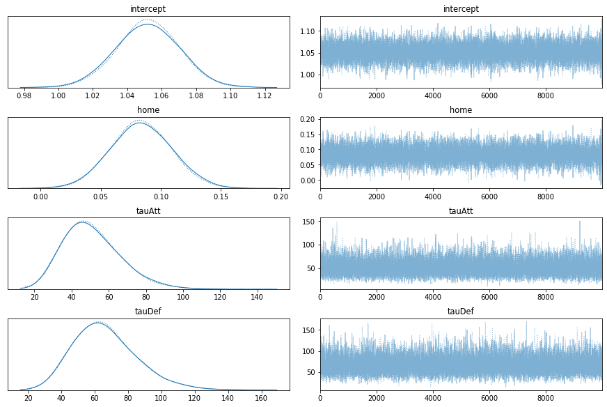
pm.summary(trace, var_names=['intercept', 'home', 'tauAtt', 'tauDef'])
| mean | sd | hpd_3% | hpd_97% | mcse_mean | mcse_sd | ess_mean | ess_sd | ess_bulk | ess_tail | r_hat | |
|---|---|---|---|---|---|---|---|---|---|---|---|
| intercept | 1.052 | 0.018 | 1.018 | 1.086 | 0.000 | 0.000 | 20293.0 | 20293.0 | 20286.0 | 14523.0 | 1.0 |
| home | 0.084 | 0.025 | 0.037 | 0.131 | 0.000 | 0.000 | 20294.0 | 18719.0 | 20305.0 | 12261.0 | 1.0 |
| tauAtt | 51.271 | 15.266 | 24.746 | 79.821 | 0.097 | 0.071 | 24849.0 | 23229.0 | 24757.0 | 16822.0 | 1.0 |
| tauDef | 66.623 | 19.002 | 34.314 | 103.936 | 0.117 | 0.085 | 26570.0 | 25032.0 | 26125.0 | 16042.0 | 1.0 |
varNames = ['intercept', 'home', 'tauAtt', 'tauDef']

samples = np.empty((20000, 4))
for ii, var in enumerate(varNames):
    samples[:,ii] = trace[var]

_ = corner.corner(samples, labels=varNames, lw=2, hist_kwargs={"lw" : 2}, show_titles=True)
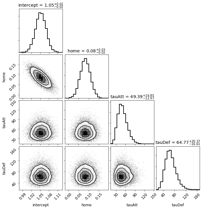
It appears that the only significant correlations are between the intercept term and the home ice advantage term. This correlation makes sense, however, given that the intercept effectively quantifies the typical number of log goals (typical goals = exp(intercept)) scored by a team. If the average team scores more goals, we would expect the home ice advantage to weaken.
Now let’s consider the Bayesian fraction of missing information (BFMI), the Gelman-Rubin statistic, and the marginal energy distribution of the MCMC. I won’t go into the math here, but we want the BFMI and Gelman-Rubin statistics to be about 1 for a converged chain. Furthermore, if the distribution of marginal energy and the energy transition are similar, the chain has likely converged.
# Estimate the maximum Bayesian fraction of missing information (BFMI) and
# Gelman-Rubin statistic
bfmi = np.max(pm.stats.bfmi(trace))
maxGR = max(np.max(gr) for gr in pm.stats.rhat(trace).values()).values
print("Rhats:", pm.stats.rhat(trace).values())
Rhats: ValuesView(<xarray.Dataset>
Dimensions:         (attsStar_dim_0: 31, atts_dim_0: 31, defsStar_dim_0: 31, defs_dim_0: 31)
Coordinates:
  * attsStar_dim_0  (attsStar_dim_0) int64 0 1 2 3 4 5 6 ... 25 26 27 28 29 30
  * defsStar_dim_0  (defsStar_dim_0) int64 0 1 2 3 4 5 6 ... 25 26 27 28 29 30
  * atts_dim_0      (atts_dim_0) int64 0 1 2 3 4 5 6 7 ... 24 25 26 27 28 29 30
  * defs_dim_0      (defs_dim_0) int64 0 1 2 3 4 5 6 7 ... 24 25 26 27 28 29 30
Data variables:
    home            float64 1.0
    intercept       float64 1.001
    attsStar        (attsStar_dim_0) float64 1.0 0.9999 1.0 1.0 ... 1.0 1.0 1.0
    defsStar        (defsStar_dim_0) float64 1.0 1.0 1.0 1.001 ... 1.0 1.0 1.0
    tauAtt          float64 1.0
    tauDef          float64 1.0
    atts            (atts_dim_0) float64 1.0 1.0 1.0 1.0 ... 1.0 1.001 1.0 1.0
    defs            (defs_dim_0) float64 1.0 1.0 1.0 1.0 1.0 ... 1.0 1.0 1.0 1.0)
ax = pm.energyplot(trace, kind="histogram", legend=True, figsize=(6, 4))
ax.set_title("BFMI = %lf\nGelman-Rubin = %lf" % (bfmi, maxGR));
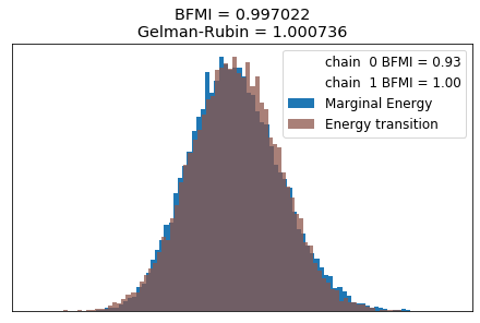
It looks like our model has converged!
Explore model implications
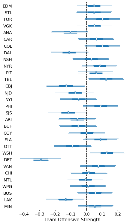
Now we can examine the inferred posterior distributions for our model latent variables like a team’s attack and defense strengths.
ax = pm.forestplot(trace, var_names=['atts'])
ax[0].set_yticklabels(teams.iloc[::-1]['name'].tolist())
ax[0].axvline(0, color="k", zorder=0, ls="--")
ax[0].set_xlabel('Team Offensive Strength', fontsize=15)
ax[0].set_title("");
ax = pm.forestplot(trace, var_names=['defs'])
ax[0].axvline(0, color="k", zorder=0, ls="--")
ax[0].set_yticklabels(teams.iloc[::-1]['name'].tolist())
ax[0].set_xlabel('Team Defensive Strength', fontsize=15)
ax[0].set_title("");
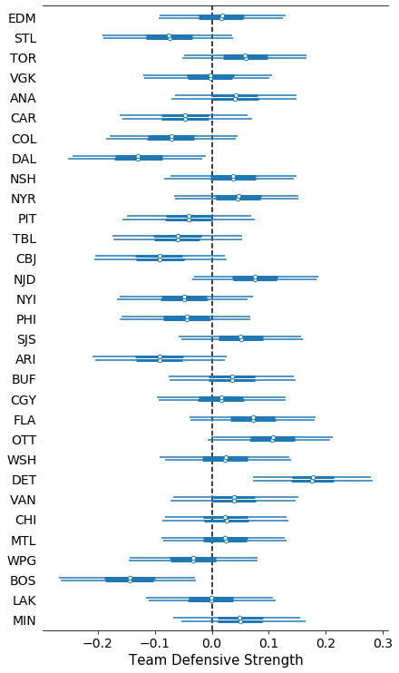
Now let’s plot these same quantities, but ranking teams from worst (DET) to best. Remember: a team wants to have a large attack strength (score more goals!) and a large negative defense strength (make the other team score fewer goals!).
# Calculate median, 68% CI for atts, defs for each team
medAtts = np.median(trace["atts"], axis=0)
medDefs = np.median(trace["defs"], axis=0)

defsCI = pm.stats.hpd(trace["defs"], credible_interval=0.68)
attsCI = pm.stats.hpd(trace["atts"], credible_interval=0.68)
# Plot ordered attacking strength
fig, ax = plt.subplots(figsize=(10,4))

# Order values by worst to best attacking
inds = np.argsort(medAtts)

x = np.arange(len(medAtts))
ax.errorbar(x, medAtts[inds], yerr=[medAtts[inds] - attsCI[inds,0], attsCI[inds,1] - medAtts[inds]],
            fmt='o')

ax.axhline(0, lw=2, ls="--", color="k", zorder=0)
ax.set_title('68% Confidence Interval of Attack Strength, by Team')
ax.set_xlabel('Team')
ax.set_ylabel('Posterior Attack Strength\n(Above 0 = Good)')
_ = ax.set_xticks(x)
_ = ax.set_xticklabels(teams["name"].values[inds], rotation=45)
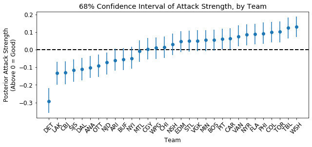
From this season’s results, my model infers that the five best offensive teams are WSH, TBL, TOR, COL, and PHI whereas the worst 5 teams are DET, LAK, CBJ, SJS, and DAL.
# Plot ordered defense strength
fig, ax = plt.subplots(figsize=(10,4))

# Order values by worst to best attacking
inds = np.argsort(medDefs)[::-1]

x = np.arange(len(medDefs))
ax.errorbar(x, medDefs[inds], yerr=[medDefs[inds] - defsCI[inds,0], defsCI[inds,1] - medDefs[inds]],
            fmt='o')

ax.axhline(0, lw=2, ls="--", color="k", zorder=0)
ax.set_title('68% Confidence Interval of Defense Strength, by Team')
ax.set_xlabel('Team')
ax.set_ylabel('Posterior Defense Strength\n(Below 0 = Good)')
_ = ax.set_xticks(x)
_ = ax.set_xticklabels(teams["name"].values[inds], rotation=45)
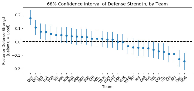
My model infers that the five best defensive teams are BOS, DAL, ARI, CBJ, and STL whereas the five worst defensive teams are DET, OTT, NJD, FLA, and TOR.
Below, I’ll see how teams’ points percentage varies as a function of attack and defense strengths. I expect that teams with a higher points percentage, e.g. BOS and STL, will have large attack and large negative defense strengths and for the converse to be true for bad teams like DET.
fig, ax = plt.subplots(figsize=(6,5))

im = ax.scatter(medDefs, medAtts, c=pointsArr, s=60, zorder=1)
ax.axhline(0, lw=1.5, ls="--", color="grey", zorder=0)
ax.axvline(0, lw=1.5, ls="--", color="grey", zorder=0)

cbar = fig.colorbar(im)
cbar.set_label(r"Points % as of March 12$^{\mathrm{th}}$", fontsize=15)
ax.set_xlabel('Posterior Defense Strength', fontsize=15)
ax.set_ylabel('Posterior Attack Strength', fontsize=15)
ax.set_xlim(-0.2, 0.2);
ax.set_ylim(-0.32, 0.15);
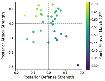
Above I plotted each team’s posterior attack strength vs. the posterior defense strength. Each point represents a team and the color encodes the team’s season points total as of March 12th, 2020 when the NHL season was officially suspended. Clearly, there is a gradient in total points (color) that follows a reasonable trend: teams with strong attacks (large attack strength) and strong defense (large negative defense strength) tend to perform bettern and accumulate more points. BOS, arguably the best team in the NHL in 2019-2020, is located in the strong attack/defense quandrant and is appropriately colored yellow for 100 points. DET (purple dot in the bad quadrant), on the other hand, is far-and-away the worst team in the NHL and our model captures that.
fig, ax = plt.subplots(figsize=(6,5))

im = ax.scatter(medAtts, goalsFor, c=pointsArr, s=60, zorder=1)
ax.axhline(np.mean(goalsFor), lw=1.5, ls="--", color="grey", zorder=0)
ax.axvline(0, lw=1.5, ls="--", color="grey", zorder=0)

cbar = fig.colorbar(im)
cbar.set_label(r"Point % as of March 12$^{\mathrm{th}}$", fontsize=15)
ax.set_xlabel('Posterior Attack Strength', fontsize=15)
ax.set_ylabel('Goals For Per Game', fontsize=15);
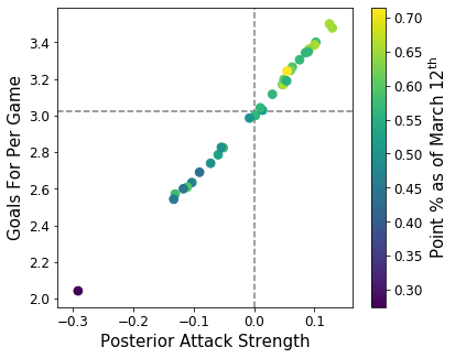
It looks like our posterior attack strength parameter accurately captures offense strength as there is a tight correlation between the two. Generally, it appears the number of points a team earns increases with both posterior attack strength and goals for as we’d expect, but there is some scatter that is likely caused by the uncertainty in the posterior distributions.
fig, ax = plt.subplots(figsize=(6,5))

im = ax.scatter(medAtts, goalsAgainst, c=pointsArr, s=60, zorder=1)
ax.axhline(np.mean(goalsAgainst), lw=1.5, ls="--", color="grey", zorder=0)
ax.axvline(0, lw=1.5, ls="--", color="grey", zorder=0)

cbar = fig.colorbar(im)
cbar.set_label(r"Point % as of March 12$^{\mathrm{th}}$", fontsize=15)
ax.set_xlabel('Posterior Defense Strength', fontsize=15)
ax.set_ylabel('Goals Against Per Game', fontsize=15);
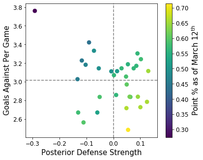
Interestingly, the correlation between goals against and posterior defense strength is much weaker than what we saw above for attacking values. The correlation between points and a linear combination of goals against and posterior defense strength, i.e. the color gradient from the top left to the bottom right of the figure, appears much stronger. Perhaps there’s more to defense than simply goals conceded. I think this makes sense in a game like hockey because a team can get shelled 50-15 in terms of shots but only lose 1-0 whereas a team can lose 3-0 but take more shots than the other team and dominate the play. Hockey is a non-linear game to say the least, but I think our model is doing pretty well given its simplicity.
Model Implications for Coach Strategies
We can use our inferred offensive and defensive team strengths to help inform a coach’s strategy for a given matchup. Consider the case wherein a team with a strong attack, e.g. TBL or TOR, plays a team with a weak defense, e.g. DET. In this case, it would make sense for the strong attacking team to focus more on their offensive output to exploit the defensive weakness of their opponent and give themselves the best chance of winning the game. For teams like TOR that are fighting to keep a playoff spot, the 3rd spot in the division in TOR’s case, adopting such strategies to maximize earned points is essential to making the playoffs.
Simulating games (and the rest of the 2019-2020 season)
I have shown with fairly high confidence that the defending champions, the St. Louis Blues, are a much better offensive and defensive team than the Chicago Blackhawks. Also, Detroit is a bad team overall (other than former Blue Note Robby Fabbri and their likely future captain Dylan Larkin). Therefore, it appears that my model is realistically modeling the strengths and weaknesses of NHL teams given the games we have observed so far and our simplified model. Now we can turn to making some predictions using simulations.
My favorite aspect of probabilistic modeling is how I can draw samples from the posterior distribution to simulate games and reasonably account for model uncertainty and are consistent with the observed results of the NHL regular season. That is, I can estimate the likelihood that NHL Team A beats Team B at home given their previous performances. Moreover, I can estimate probability distributions for the score. Naturally, this can be extrapolated to simulating “Best-of-7” series and the playoffs more generally. For now, I will focus on simulating individual games and then the rest of the season to see how many points each team likely would have earned throughout a full 82 game season. Recall that above, I saved the entire season’s schedule. We will use that below to simulate the rest of the season.
Below, I define a simple function that draws a sample from the posterior distribution and uses that to simulate a regular season NHL game, including those that go into overtime (OT). Moreover, recall that above I calculated the empirirical probability that a game goes into a shootout (SO) given OT. I use that below to decide how games end.
def simulateGame(trace, ind, homeTeam, awayTeam, teams, chain=0):
    """
    Simulate an NHL game where awayTeam plays at homeTeam and trace
    is a draw from the posterior distribution for model parameters,
    e.g. atts and defs. In this simplified model, if the game goes to
    OT, I say the game goes to a SO 34.4% of the team, the empirical
    fraction from this season's NHL results. If the game ends in either
    and OT or SO, I assign each team equal odds to win and randomly decide,
    assigning an extra goal to the winner.

    Parameters
    ----------
    trace : iterable
        Posterior distribution MCMC chain
    ind : int
        Index representing posterior draw
    homeTeam : str
        Name of the home team, like STL
    awayTeam : str
        Name of the away team, like CHI
    teams : pd.DataFrame
        pandas dataframe of teams that maps
        team name to a unique index
    chain : int (optional)
        Which chain to draw from. Defaults to 0.

    Returns
    -------
    homeGoals : int
        number of goals scored by the home team
    awayGoals : int
        number of goals scored by the away team
    homeWin : bool
        whether or not the hometeam won
    homePoints : int
        number of standings points earned by home team
    awayPoints : int
        number of standings points earned by away team
    note : str
        indicates if the game finished in regulation (REG),
        overtime (OT), or a shooutout (SO).
    """

    # Extract posterior parameters
    home = trace.point(ind, chain=chain)["home"]
    intercept = trace.point(ind)["intercept"]
    homeAtt = trace.point(ind)["atts"][int(teams[teams["name"] == homeTeam]["ind"])]
    homeDef = trace.point(ind)["defs"][int(teams[teams["name"] == homeTeam]["ind"])]
    awayAtt = trace.point(ind)["atts"][int(teams[teams["name"] == awayTeam]["ind"])]
    awayDef = trace.point(ind)["defs"][int(teams[teams["name"] == awayTeam]["ind"])]

    # Compute home and away goals using log-linear model, draws for model parameters
    # from posterior distribution. Recall - model goals as a draws from
    # conditionally-independent Poisson distribution: y | theta ~ Poisson(theta)
    homeTheta = np.exp(home + intercept + homeAtt + awayDef)
    awayTheta = np.exp(intercept + awayAtt + homeDef)
    homeGoals = np.random.poisson(homeTheta)
    awayGoals = np.random.poisson(awayTheta)

    # Figure out who wins
    note = "REG"
    if homeGoals > awayGoals:
        homeWin = True
        homePoints = 2
        awayPoints = 0
    elif awayGoals > homeGoals:
        homeWin = False
        awayPoints = 2
        homePoints = 0
    # Overtime!
    else:
        # Each team gets at least 1 point now
        homePoints = 1
        awayPoints = 1

        # Does the game go into a shootout?
        if np.random.uniform(low=0, high=1) < 0.344:
            note = "SO"
            # Randomly decided who wins
            if np.random.uniform(low=0, high=1) < 0.5:
                homeWin = True
                homeGoals += 1
                homePoints = 2
            else:
                homeWin = False
                awayGoals += 1
                awayPoints = 2
        # No shootout, randomly decide who wins OT
        else:
            note = "OT"
            # Randomly decided who wins
            if np.random.uniform(low=0, high=1) < 0.5:
                homeWin = True
                homeGoals += 1
                homePoints = 2
            else:
                homeWin = False
                awayGoals += 1
                awayPoints = 2

    return homeGoals, awayGoals, homeWin, homePoints, awayPoints, note
Case Study: How likely is it that the St. Louis Blues sweep the season series against the Chicago Blackhawks, a team that has not won a game in the playoffs since 2016?
This season, the Blues swept the season series with Chicago, 4 wins to 0 losses, for the first time in franchise history. Using my model, I can estimate how often that would have occured if we could replay the season an arbitrary number of times. For this estimation, I’ll simulate 2,500 4 games series where each team has 2 home games.
nTrials = 2500
nGames = 4

# numpy array to hold results
bluesRes = np.zeros((nTrials, nGames), dtype=int)

# random array of indicies to sample from
choices = np.arange(10000)

for ii in range(nTrials):

    # nGames game series
    for jj in range(nGames):

        # Set home, away team
        if jj < 2:
            homeTeam = "STL"
            awayTeam = "CHI"
        else:
            homeTeam = "CHI"
            awayTeam = "STL"

        # Draw random sample with replacement from one of 2 MCMC chains
        ind = np.random.choice(choices)
        chain = np.random.randint(2)

        # Simulate the game, save whether or not Blues won the game
        _, _, homeWin, _, _, _ = simulateGame(trace, ind, homeTeam, awayTeam, teams, chain=chain)
        if jj < 2:
            bluesRes[ii, jj] = int(homeWin)
        else:
            bluesRes[ii, jj] = int(not homeWin)
mask = bluesRes.all(axis=1)
print("STL sweeps the season series against CHI in %0.1lf %% of simulated seasons." % (np.mean(mask) * 100))

mask = (bluesRes.sum(axis=1) > 2)
print("STL wins the season series against CHI in %0.1lf %% of simulated seasons." % (np.mean(mask) * 100))

mask = (bluesRes.sum(axis=1) == 2)
print("STL ties the season series against CHI in %0.1lf %% of simulated seasons." % (np.mean(mask) * 100))

mask = (bluesRes.sum(axis=1) < 2)
print("CHI wins the season series against STL in %0.1lf %% of simulated seasons." % (np.mean(mask) * 100))
STL sweeps the season series against CHI in 9.9 % of simulated seasons.
STL wins the season series against CHI in 42.2 % of simulated seasons.
STL ties the season series against CHI in 35.5 % of simulated seasons.
CHI wins the season series against STL in 22.2 % of simulated seasons.
Awesome! It was of course unlikely for the Blues to sweep the regular season series against the Blackhawks since they were not that bad this year, but the Blues had a decent chance, about 1 in 10, and took it. My model predicts that the Blues should win, or at least tie, the season series over 3/4s of the time.
Simulating the 2019-2020 season up until the season suspension
Now that I think the model is working well, I’m going to perform one final validation before I simulate the final season standings and the playoffs. I will replay the season up until it was suspended using draws from the posterior distribution. If my model is working, I’d hope that a team’s expected points is nearly the same as how many points they actually scored.
I’ll select which games were played and use this schedule to re-simulate the played regular season.
playedSchedule = schedule.iloc[schedule.index < datetime(2020, 3, 12)]
playedSchedule.tail()
| homeTeam | awayTeam | |
|---|---|---|
| Date | ||
| 2020-03-11 | ANA | STL |
| 2020-03-11 | CHI | SJS |
| 2020-03-11 | COL | NYR |
| 2020-03-11 | EDM | WPG |
| 2020-03-11 | LAK | OTT |
Now I can run some simulations and here I outline my simulation procedure. For each iteration, I will make one draw from the posterior distribution for each team, i.e. each game will be played with the same home, intercept, attack strengths, and defense strenghts that were drawn from the posterior distribution for each team (except only one draw for home and intercept terms since they are the same for each team). I will then call the simulateGame function I wrote above for each game and record an estimate for the number of points earned by each team. Each team will have a column and each row will represent a season. I’ll run 1,000 simulations so I can derive reasonable marginal posterior distributions for each team’s expected points.
# Number of seasons to simulate
numSeasons = 1000

res = list()
for ii in range(numSeasons):

    # Draw random sample with replacement from one of 2 MCMC chains
    ind = np.random.choice(choices)
    chain = np.random.randint(2)

    # Teams start season with 0 points
    tmpPoints = np.zeros(len(teams))
    for jj in range(len(playedSchedule)):
        # Select home, away teams
        homeTeam = playedSchedule.iloc[jj]["homeTeam"]
        awayTeam = playedSchedule.iloc[jj]["awayTeam"]

        # Simulate jjth game, store results
        _, _, _, homePoints, awayPoints, _ = simulateGame(trace, ind, homeTeam, awayTeam, teams, chain=chain)

        tmpPoints[int(teams[teams["name"] == homeTeam]["ind"])] += homePoints
        tmpPoints[int(teams[teams["name"] == awayTeam]["ind"])] += awayPoints

    # Save season result
    res.append(list(tmpPoints))

# Turn simulations into a dataframe as described above
playedPoints = pd.DataFrame.from_records(res, columns=teams["name"].values)
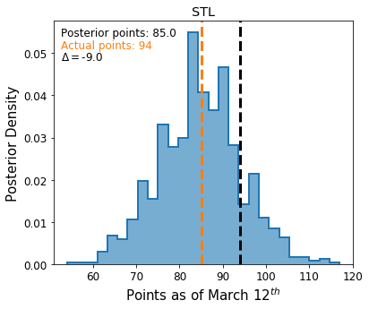
Now that we’ve simulated the season a large number of times, I will plot the inferred posterior distribution for each team’s earned standings points. First, I’ll plot these quantities for the Blues, then I’ll do the same for every other team.
fig, ax = plt.subplots(figsize=(6,5))

ax.hist(playedPoints["STL"], color="C0", bins="auto", histtype="step", lw=2, density=True)
ax.hist(playedPoints["STL"], color="C0", bins="auto", alpha=0.6, density=True)

ax.axvline(np.median(playedPoints["STL"]), color="C1", lw=3, ls="--")
ax.axvline(points["STL"], color="k", lw=3, ls="--")

ax.text(0.025, 0.95,'Posterior points: %0.1lf' % np.median(playedPoints["STL"]),
        horizontalalignment='left', color="k",
        verticalalignment='center',
        transform = ax.transAxes)

ax.text(0.025, 0.9,'Actual points: %d' % points["STL"],
        horizontalalignment='left', color="C1",
        verticalalignment='center',
        transform = ax.transAxes)

ax.text(0.025, 0.85,r'$\Delta=$%0.1lf' % (np.median(playedPoints["STL"]) - points["STL"]),
        horizontalalignment='left',
        verticalalignment='center',
        transform = ax.transAxes)

ax.set_title("STL")
ax.set_ylabel("Posterior Density", fontsize=15)
ax.set_xlabel("Points as of March 12$^{th}$", fontsize=15);
fig, axes = plt.subplots(ncols=6, nrows=5, sharex=True, figsize=(12, 11))

teamNames = list(teams["name"])
teamNames.remove("STL")
teamNames = list(np.sort(teamNames))

for ii, ax in enumerate(axes.flatten()):

    # Get team name
    teamName = teamNames[ii]

    # Turn off all y ticks, set common x range
    ax.set_yticklabels([])
    ax.set_xlim(30, 120)

    # Histogram of posterior points
    ax.hist(playedPoints[teamName], color="C0", bins="auto", histtype="step", lw=1.5, density=True)
    ax.hist(playedPoints[teamName], color="C0", bins="auto", alpha=0.6, density=True)

    # Plot observed, median posterior points
    ax.axvline(np.median(playedPoints[teamName]), color="k", lw=2, ls="--")
    ax.axvline(points[teamName], color="C1", lw=2, ls="--")

    # Annotate with actual points, posterior points, and the difference (delta)
    if points[teamName] < 70:
        offset = 0.6
    else:
        offset = 0

    ax.text(0.025 + offset, 0.925, '%d' % np.median(playedPoints[teamName]),
            horizontalalignment='left', color="k",
            verticalalignment='center', fontsize=11.5,
            transform = ax.transAxes)
    ax.text(0.025 + offset, 0.8, '%d' % points[teamName],
            horizontalalignment='left', color="C1",
            verticalalignment='center', fontsize=11.5,
            transform = ax.transAxes)
    ax.text(0.025 + offset, 0.7 ,r'$\Delta=$%d' % (np.median(playedPoints[teamName]) - points[teamName]),
            horizontalalignment='left', fontsize=11.5,
            verticalalignment='center',
            transform = ax.transAxes)
    ax.set_title(teamName)

# Format
axes[2,0].set_ylabel("Posterior Density", fontsize=25, position=(0, 0.5));
axes[4,2].set_xlabel("Points as of March 12$^{th}$", fontsize=25, position=(1, 0));
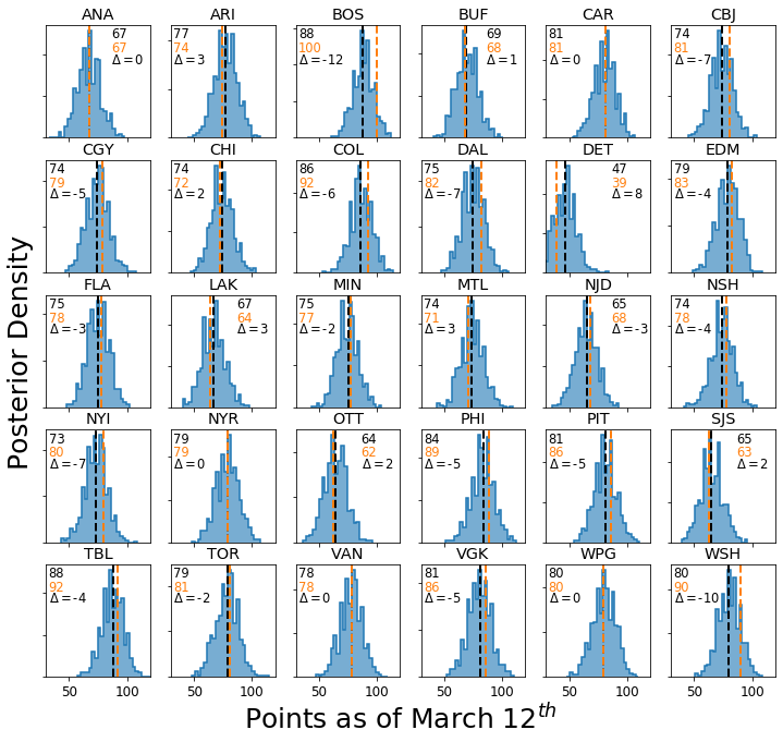
It appears that my model does a pretty good job at reproducing the 2019-2020 regular season! The median posterior points predicted by my model is dead on for WPG, VAN, NYR, ANA, and CAR. Moreover, it is within a few points many teams (average error of 4 points, or 2 regular wins), so I think that I can conclude that my model is actually picking up on how good teams are and appropriately modeling the results of games for this season.
It does appear, however, that my model underpredicts the points earned by the best teams, e.g. BOS, WSH, and STL. Furthermore, my model overpredicts the points earned by the worst team, DET. This effect is a consequence of the well-known effect of shrinkage. Shrinkage oftens occurs for hierarchical Bayesian models and both Baio and Blangiardo and Daniel Weitzenfeld’s great write-up describe this effect in detail, so please see their write-ups for an in-depth discussion.
Basically, what’s happening is that our hyperprior for attack and defense strengths has a prior mean of 0. This in effect pulls each teams strengths towards 0, depending on their observed scoring rates, effectively acting as a regularization term. Baio and Blangiardo explain how using different hyperpriors for different classes of teams, e.g. one for the good(likely playoff) teams, one for the average (wildcard playoff teams, those that almost make the playoffs) teams, and one for bad teams like DET and OTT, can mitigate shrinkage. Personally, I like including forms of regularization in my models to prevent observing too many extreme results, so I will keep it in.
Simulating the unplayed games of the 2019-2020 NHL season
I am convinced that my model does a good job of reproducing the results of the 2019-2020 NHL season up until the season was suspended. Moreover, the latent parameters inferred by my model, i.e. each team’s attack and defense strength, appears to provide reasonable approximations for a team’s scoring and defensive performance. Given a working model, I can now use it to predict the final standings for the season to see where teams would end up in the playoffs! To do that, I will simulate the rest of the season, similar to my simulations above, and add those results to the observed points each team had accrued so far. Then, for simplicity, I will sort teams by point percentage to determine who makes the playoffs and what seed they earned. Note that future work should more robustly track game-by-game results to figure out tie breaker scenarios. Note that my model can do that, I’m just taking a simpler approach.
futureSchedule = schedule.iloc[schedule.index >= datetime(2020, 3, 12)]
futureSchedule.tail()
| homeTeam | awayTeam | |
|---|---|---|
| Date | ||
| 2020-04-04 | NYR | CHI |
| 2020-04-04 | OTT | PIT |
| 2020-04-04 | SJS | ANA |
| 2020-04-04 | TOR | MTL |
| 2020-04-04 | VAN | VGK |
# Number of seasons to simulate
numSeasons = 100

res = list()
for ii in range(numSeasons):

    # Draw random sample with replacement from one of 2 MCMC chains
    ind = np.random.choice(choices)
    chain = np.random.randint(2)

    # Teams start season with 0 points
    tmpPoints = np.zeros(len(teams))
    for jj in range(len(futureSchedule)):
        # Select home, away teams
        homeTeam = futureSchedule.iloc[jj]["homeTeam"]
        awayTeam = futureSchedule.iloc[jj]["awayTeam"]

        # Simulate jjth game, store results
        _, _, _, homePoints, awayPoints, _ = simulateGame(trace, ind, homeTeam, awayTeam, teams, chain=chain)

        tmpPoints[int(teams[teams["name"] == homeTeam]["ind"])] += homePoints
        tmpPoints[int(teams[teams["name"] == awayTeam]["ind"])] += awayPoints

    # Save season result
    res.append(list(tmpPoints))

# Turn simulations into a dataframe as described above
futurePoints = pd.DataFrame.from_records(res, columns=teams["name"].values)
We’ve simulated the rest of the season. Now, we can add each team’s earned points to the posterior future points to estimate a posterior probability distribution for how many points a team would have earned by the end of the season. Then, I can compute the mean of these distribution and sort the teams to see who would have likely earned the President’s Trophy.
# Calculate posterior for end of season points
totalPoints = futurePoints.copy()
teamNames = list(teams["name"])
teamNames = list(np.sort(teamNames))

for team in teamNames:
    totalPoints[team] += points[team]
meanTotal = totalPoints.mean(axis=0).sort_values(ascending=False)
meanTotal
BOS    115.49
TBL    108.15
COL    107.80
WSH    106.81
STL    106.65
PHI    104.74
PIT    100.89
VGK     97.99
DAL     97.39
CAR     97.34
EDM     95.64
TOR     94.98
NYI     94.91
CBJ     92.85
VAN     92.47
FLA     92.38
CGY     92.28
WPG     91.49
NSH     91.27
NYR     91.23
MIN     90.86
ARI     87.87
CHI     85.15
MTL     82.75
BUF     80.76
NJD     80.29
ANA     77.42
LAK     75.75
SJS     72.98
OTT     70.90
DET     44.85
dtype: float64
It looks like BOS would have won the Presidents’ Trophy. Congrats! Pretty much like winning the Cup, right? I am a bit sad, but ultimately not surprised, to see COL finish ahead of STL. COL was a wagon over the stretch and it would have been a tight finish with STL.
Who Makes the Playoffs?
# Divisions
central = ["STL", "CHI", "MIN", "DAL", "NSH", "WPG", "COL"]
pacific = ["SJS", "LAK", "ANA", "CGY", "EDM", "VGK", "VAN", "ARI"]
metro = ["WSH", "PHI", "PIT", "CAR", "CBJ", "NYI", "NYR", "NJD"]
atlantic = ["BOS", "TBL", "TOR", "FLA", "MTL", "BUF", "OTT", "DET"]

# Conferences
west = central + pacific
east = metro + atlantic

# Compute posterior standings
centralStandings = totalPoints[central].mean(axis=0).sort_values(ascending=False)
pacificStandings = totalPoints[pacific].mean(axis=0).sort_values(ascending=False)
metroStandings = totalPoints[metro].mean(axis=0).sort_values(ascending=False)
atlanticStandings = totalPoints[atlantic].mean(axis=0).sort_values(ascending=False)
westStandings = totalPoints[west].mean(axis=0).sort_values(ascending=False)
eastStandings = totalPoints[east].mean(axis=0).sort_values(ascending=False)
Central Division Final Standings
centralStandings
COL    107.80
STL    106.65
DAL     97.39
WPG     91.49
NSH     91.27
MIN     90.86
CHI     85.15
dtype: float64
Pacific Division Final Standings
pacificStandings
VGK    97.99
EDM    95.64
VAN    92.47
CGY    92.28
ARI    87.87
ANA    77.42
LAK    75.75
SJS    72.98
dtype: float64
Metro Division Final Standings
metroStandings
WSH    106.81
PHI    104.74
PIT    100.89
CAR     97.34
NYI     94.91
CBJ     92.85
NYR     91.23
NJD     80.29
dtype: float64
Atlantic Division Final Standings
atlanticStandings
BOS    115.49
TBL    108.15
TOR     94.98
FLA     92.38
MTL     82.75
BUF     80.76
OTT     70.90
DET     44.85
dtype: float64
Western Conference Final Standings
westStandings
COL    107.80
STL    106.65
VGK     97.99
DAL     97.39
EDM     95.64
VAN     92.47
CGY     92.28
WPG     91.49
NSH     91.27
MIN     90.86
ARI     87.87
CHI     85.15
ANA     77.42
LAK     75.75
SJS     72.98
dtype: float64
The Western Conference 1 and 2 wildcard teams are CGY and WPG, respectively.
Eastern Conference Final Standings
eastStandings
BOS    115.49
TBL    108.15
WSH    106.81
PHI    104.74
PIT    100.89
CAR     97.34
TOR     94.98
NYI     94.91
CBJ     92.85
FLA     92.38
NYR     91.23
MTL     82.75
BUF     80.76
NJD     80.29
OTT     70.90
DET     44.85
dtype: float64
The Eastern Conference 1 and 2 wildcard teams are CAR and NYI, respectively.
Predicted Playoff Matchups
From the posterior distributions summarized in the above tables, we can see what playoff matchups are most likely according to my model and given the current season results.
Western Conference
COL vs (WC2) WPG
VGK vs (WC1) CAL
STL vs DAL
EDM vs VAN
In this case although I like Vegas, I’d be pulling for both CAL and EDM so we would have a “Battle of Alberta” matchup in the second round. I never like playing DAL in the playoffs, especially since they now have several axes to grind against the Blues, but I’m sure it’d be an exciting series.
Eastern Conference
BOS vs (WC2) NYI
WSH vs (WC1) CAR
TBL vs TOR
PHI vs PIT
Although I would prefer the drama of another BOS vs TOR 1st round matchup, I think these would all be excellent series. WSH vs CAR 1st round rematch, the PHI vs PIT eternal grudge-match, and a TBL vs TOR matchup that would likely yield tons of goals.